Aymen Hafeez

$\newcommand{\dd}{\mathrm{d}}$

We’ll use some of the techniques demonstrated in the other examples to expand on how we can leverage matplotlib’s builtin functionality with animplotlib to create some cool looking animations.

In a previous post we made an animation of the Lorenz attractor. Here we’ll be looking at the Dadras attractor. The Dadras attractor differs from the Lorenz attractor in that it displays a winged, or multi-scrolled shaped when plotted. It can be described by the following set of nonlinear differential equations:

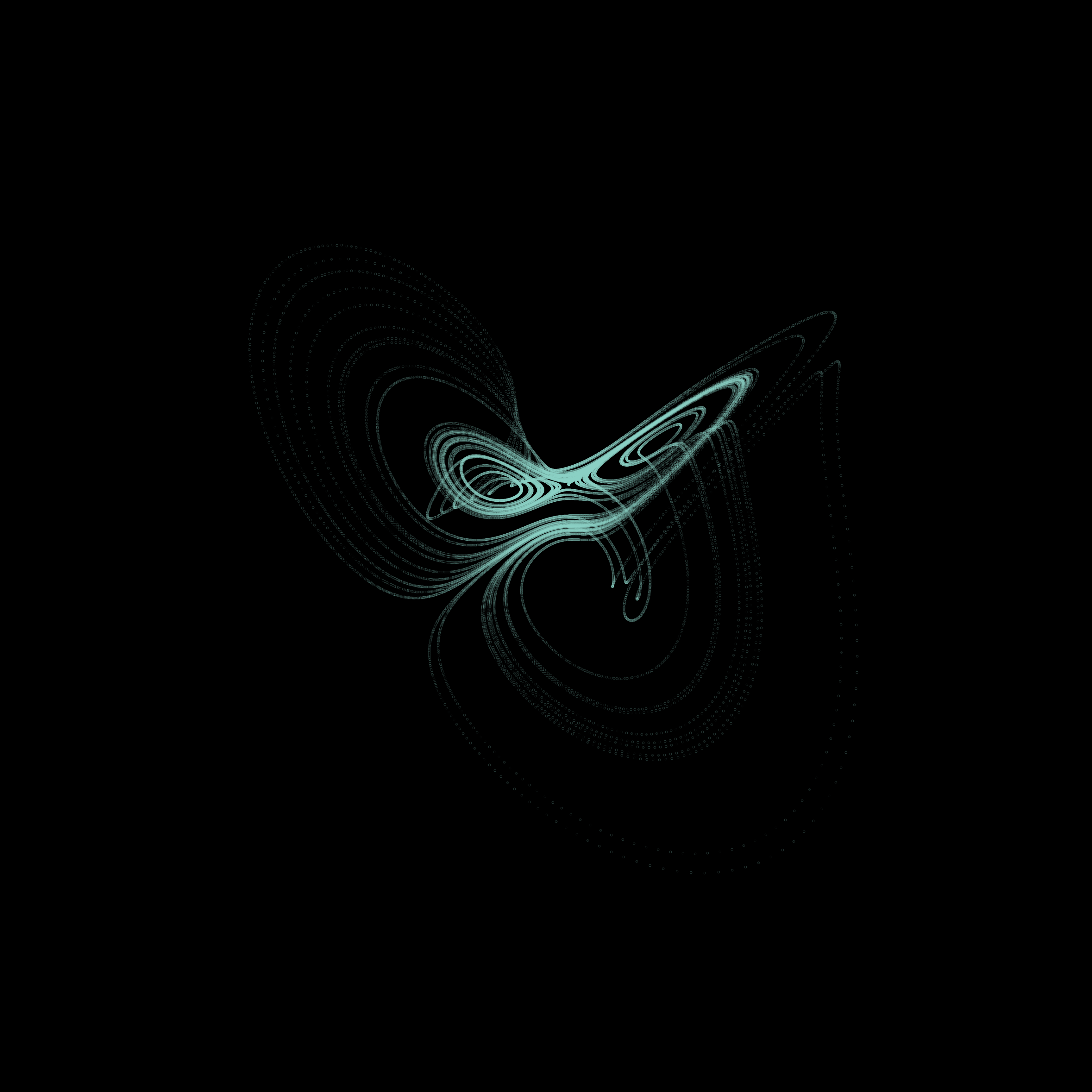
A common parameter configuration for the Dadras attractor to display the multi-scrolled shape shown above is $a=3, b=2.7, c=1.7, d=2, e=9$

In the example animating the Lorenz attractor we solved the system for a variety of initial conditions and plotted the solutions on a single axes to visualise how chaotic systems are sensitive to their input parameters. Here, rather than varying the parameters being input into the system we define we’ll vary some of the parameters that can be set within matplotlib to customise the appearance of the animation.

First we’ll import the necessary libraries and define the Dadras system:

import numpy as np
import matplotlib.pyplot as plt
from scipy.integrate import odeint
import animplotlib as anim

# Set time interval and initial conditions
t = np.linspace(0, 75, 10000)
x0 = [1.1, 2.1, -2]


# Define the Dadras system
def dadras(x_var, t, a, b, c, d, e):
    x, y, z = x_var
    dxdt = y - a * x + b * y * z
    dydt = c * y - x * z + z
    dzdt = d * x * y - e * z
    return [dxdt, dydt, dzdt]


# Solving the Dadras system
def solve_dadras(x0, t, a, b, c, d, e):
    return odeint(dadras, x0, t, args=(a, b, c, d, e))

We then call the solve_dadras function to generate the data we’re going to plot:

x_solve = solve_dadras(x0, t, a=3, b=2.7, c=1.7, d=2, e=9)
x, y, z = x_solve.T

Next, we can create a figure and axes, and empty lists for the lines, points, and $x$, $y$, and $z$ data to be added to.

plt.style.use("dark_background")
fig = plt.figure()
ax = fig.add_subplot(111, projection="3d")

lines = []
points = []
xs, ys, zs = [], [], []

Setting plt.style.use("dark_background") will help enhance the affect we’re trying to achieve. Note that this must be done before setting fig and ax in order for it to be applied to the figure and axes

Rather than generating multiple solutions with varying parameters or initial conditions, varying some of the parameters which can be passed as arguments into the axes plots can allow us to achieve some interesting looking plots. Two such arguments are linewidth and alpha. Overlaying the same plot while gradually increasing the linewidth and decreasing the alpha value can produce a glow-like affect. We first create a list of linewidth and alpha values to iterate over:

# Values for linewidth and alpha
line_config = [
    (1, 1),
    (2, 0.5),
    (3, 0.4),
    (4, 0.3),
    (6, 0.2),
    (8, 0.15),
    (9, 0.15),
    (11, 0.15),
    (13, 0.12),
    (17, 0.1),
    (20, 0.05),
]

Then, we pass the list of linewidth and alpha values to the axes, while also appending line and point plots, and (x, y, z) to the empty lists we created earlier.

# Iterating over the values for linewidth and alpha
for config in line_config:
    lw, alpha = config
    xs.append(x)
    ys.append(y)
    zs.append(z)
    # Setting linewidth and alpha to each value in the list
    line, = ax.plot([], [], [], c="lightblue", lw=lw, alpha=alpha)
    point, = ax.plot([], [], [], c="lightblue", lw=0, alpha=alpha)
    lines.append(line)
    points.append(point)

ax.set_xlim(np.min(x), np.max(x))
ax.set_ylim(np.min(y), np.max(y))
ax.set_zlim(np.min(z), np.max(z))
ax.set_axis_off()

# Calling the AnimPlot3D class
anim.AnimPlot3D(fig, [ax] * len(lines), lines, points, xs, ys, zs,
                plot_speed=20, rotation_speed=0.036, l_num=1500)

What we’re seeing in the animation is just the same plot being animated over itself, but each with a slightly thicker line and slightly higher alpha value.

Back to examples