Heat conduction in a symmetric, finite rod
Deriving an expression for the temperature profile for a symmetric, finite rod geometry.
$\newcommand{\dd}{\mathrm{d}}$
Consider the following 1-D metal bar
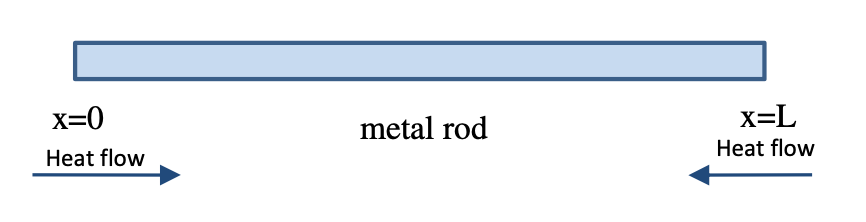
Heat flow in one dimension can be generalised by Fourier’s law, which states that heat will flow down a negative temperature gradient,
\[q = -k\frac{\dd T}{\dd x},\]where $k$ is thermal conductivity.
For a system with symmetric, finite geometry we can set the following spatial and temporal boundary conditions:
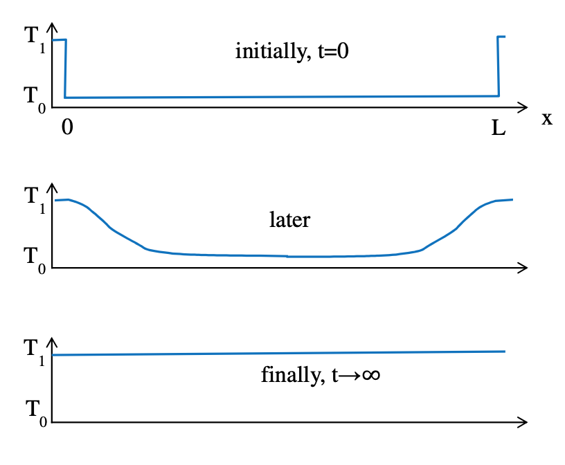
- when $x = 0, \ T = T_1$; when $x = L, \ T = T_1$
- when $t = 0, \ T = T_0$
We can derive a 1-D heat transfer equation by doing a balance over a small control volume in a short period of time $\delta t$:

The volume, $V$, can be rewritten as $A\delta x$,
\[-k\frac{\partial T}{\partial x}A\delta t - \left[-k\left(\frac{\partial T}{\partial x} + \frac{\partial^2T}{\partial x^2}\delta x\right)\right]A\delta t = \rho A \delta x c_p \Delta T\]and after some manipulation we get
\[k \frac{\partial^2T}{\partial x^2} = \rho c_p \frac{\Delta T}{\delta t}\]Taking the limit as the right hand side goes to zero,
\[k \frac{\partial^2T}{\partial x^2} = \rho c_p \frac{\partial T}{\partial t}\] \[\frac{\partial T}{\partial t} = \frac{k}{\rho c_p}\frac{\partial^2T}{\partial x^2}\]We can define thermal diffusivity $\alpha = \frac{k}{\rho c_p}$, and so we get the 1-D heat transfer equation with no internal heat generation:
\[\frac{\partial^2 T}{\partial x^2} = \frac{1}{\alpha} \frac{\partial T}{\partial t}\]In order to solve this we need to non-dimensionalise the variables involved. Let us define the following dimensionless variables:
\[\hat{T} = \frac{T - T_1}{T_0 - T_1}\] \[z = \frac{x}{L}\] \[\tau = \frac{\alpha}{L^2} t\]To write the heat equation in terms of the dimensionless variables we need to rewrite the original variables and their derivatives in terms of the dimensionless variables.
\[T = \hat{T}(T_0 - T_1) + T_1; \ \ \delta T = (T_0 - T_1)\delta \hat{T}\] \[x = Lz; \ \ \delta x = L \delta z\] \[t = \frac{L^2}{\alpha} \tau ; \ \ \delta t = \frac{L^2}{\alpha} \delta \tau\]Finding the first order partial derivative:
\[\frac{\partial T}{\partial t} = \lim_{\delta t \to 0} \left(\frac{\delta T}{\delta t}\right) = \lim_{\delta \tau \to 0} \left(\frac{(T_0 - T_1)\delta \hat{T}}{\frac{L^2}{\alpha}\delta \tau}\right) = \frac{\alpha(T_o - T_1)}{L^2} \frac{\partial \hat{T}}{\partial \tau}\]The first order derivative with respect to $x$ can be found as
\[\frac{\partial T}{\partial x} = \lim_{\delta x \to 0} \left(\frac{\delta T}{\delta x}\right) = \lim_{\delta x \to 0} \left(\frac{(T_0 - T_1)\delta \hat{T}}{L\delta z}\right) = \frac{(T_0 - T_1)}{L} \frac{\partial \hat{T}}{\partial z}\]And so the second order derivative is
\[\begin{equation*} \begin{aligned} \frac{\partial^2 T}{\partial x^2} &= \lim_{\delta x \to 0} \left(\frac{\frac{\partial T}{\partial x}|_{x+\delta x} - \frac{\partial T}{\partial x}|_x}{\delta x}\right) = \lim_{\delta x \to 0} \left(\frac{\frac{(T_0 - T_1)}{L}\left(\frac{\partial \hat{T}}{\partial z}|_{z+\delta z} - \frac{\partial \hat{T}}{\partial z}|_z\right)}{L\delta x}\right) = \frac{(T_0 - T_1)}{L^2}\frac{\partial^2 \hat{T}}{\partial z^2} \end{aligned} \end{equation*}\]Substituting this back into the original heat equation gives
\[\frac{(T_0 - T_1)}{L^2}\frac{\partial^2 \hat{T}}{\partial z^2} = \frac{1}{\alpha} \frac{\alpha(T_0 - T_1)}{L^2}\frac{\partial \hat{T}}{\partial \tau}\] \[\boxed{\frac{\partial^2 \hat{T}}{\partial z^2} = \frac{\partial \hat{T}}{\partial \tau}}\]Now, we must re-write the boundary conditions in terms of the non-dimensional variables. At the ends of the rods $T$ is always $T_1$, and so, the two spatial boundary conditions collapse to just one:
\[\hat{T}|_{z=0,1} = 0\]Just before $t=0$ the rod is at a uniform temperature, $T_0$, until the temperature of the ends of the rod is raised to $T_1$. And so the temporal boundary condition becomes
\[\hat{T}|_{\tau=0} = 1\]In order to now solve the differential equation derived above let us assume the solution is of the form
\[\hat{T}(z, \tau) = Z(z)\Theta(\tau)\]To substitute this into the non-dimensionalised 1-D heat equation we must first take the derivatives of the above
\[\frac{\partial^2 \hat{T}}{\partial z^2} = \frac{\partial^2(Z(z))}{\partial z^2}\Theta(\tau) = Z''\Theta\] \[\frac{\partial \hat{T}}{\partial \tau} = Z(z) \frac{\partial(\Theta(\tau))}{\partial \tau} = Z(z)\frac{\dd (\Theta(\tau))}{\dd \tau} = Z \Theta'\]And so, we have
\[Z\Theta' = Z''\Theta\]For the sake of later convenience let the above equal a constant $-\lambda^2$,
\[\frac{\Theta'}{\Theta} = \frac{Z''}{Z} = -\lambda^2\]We can now integrate both sides of the above by separation of variables:
\[\begin{equation*} \begin{aligned} \int \frac{\Theta'}{\Theta} &= \int \lambda^2 \dd \tau \\ \ln \Theta &= -\lambda^2 \tau + C \\ \Theta &= Ae^{-\lambda^2\tau} \end{aligned} \end{equation*}\]Using the temporal boundary condition, $\hat{T} = 1$ when $\tau = 0$, we get that $A = 1$.
For the $Z$ terms we have
\[\frac{Z''}{Z} = -\lambda^2\] \[Z'' + Z\lambda^2 = 0\]This is a general form with the general solution $Z = C_1\sin(\lambda z) + C_2\cos(\lambda z)$. We can find the constants by applying the spatial boundary conditions to the solution.
\[z = 0 \Rightarrow \hat{T} = 0 \ \therefore \ C_2 = 0\]For $C_1$ we have that when $z = 1$, $\hat{T} = 0$, and so, $C_1\sin(\lambda) = 0$ which means that $\lambda = n\pi$ for $n = 1, 2, 3, \dots$. Using the principle of superposition the overall solution must be the sum of the individual solutions,
\[Z = \sum_{n=1}^\infty C_n\sin(n\pi z)\]And so, multiplying the two functions together gives the solution,
\[\hat{T} = Z\Theta = \sum_{n=1}^\infty C_n e^{-n^2\pi^2\tau}\sin(n\pi z)\]In order to find the constants $C_1, C_2, C_3, \dots$, we need to use the temporal boundary condition:
\[\hat{T}|_{\tau=0} = 1 = \sum_{n=1}^\infty C_n\sin(n\pi z)\]Because the $\sin$ function is orthogonal we can use the property
\[\int_0^1 \sin(m\pi z)\sin(n\pi z) \ \dd z = 0,\]unless $n = m$. We can multiply both sides of the equation where the temporal boundary condition was applied by $\sin(m\pi z)$ for $m = 1, 2, 3, \dots$, and integrate both sides over $z$ from $0$ to $1$.
\[\begin{equation*} \begin{aligned} \int_0^1 \sin(m\pi z) \dd z &= \int_0^1 \sin(m\pi z)\sum_{n=1}^\infty C_n\sin(n\pi z) \dd z \\ &= \sum_{n=1}^\infty C_n\int_0^1 \sin(m\pi z)\sin(n\pi z) \dd z \end{aligned} \end{equation*}\]And so, we only get left with the terms where $n = m$, giving the following expression for the unknown coefficient:
\[C_n = \frac{\int_0^1 \sin(n\pi z)}{\int_0^1 \sin^2(n\pi z)}\]Using the identity $\sin^2(x) = \frac{1}{2}(1 - \cos(2x))$, we can evaluate the integral in the denominator as
\[\begin{equation*} \begin{aligned} \int_0^1 \sin^2(n\pi z) \ \dd z &= \frac{1}{2}\int_0^1 1 - \cos(2n\pi z) \ \dd z \\ &= \left[\frac{z}{2} - \frac{\sin(2n\pi z)}{2n\pi}\right]_0^1 \\ & = \frac{1}{2} \end{aligned} \end{equation*}\]The coefficient is, therefore,
\[\begin{equation*} \begin{aligned} C_n &= 2\int_0^1 \sin(n\pi z) \ \dd z \\ &= 2\left[-\frac{\cos(n\pi z)}{n\pi}\right] \\ &= \frac{2}{n\pi}(1 - (-1)^n) \end{aligned} \end{equation*}\]The coefficient is only non-zero for odd values of $n$, i.e. $C_1 = \frac{4}{\pi}, C_2 = 0, C_3 = \frac{4}{3\pi}, C_4 = 0, C_5 = \frac{4}{5\pi} \dots$. Substituting the coefficient back into the solution we got earlier we have
\[\hat{T} = \sum_{n=1}^\infty \frac{2}{n\pi}(1-(-1)^n) e^{-n^2\pi^2\tau} \sin(n\pi z)\] \[\hat{T} = \frac{4}{\pi}\left(e^{-\pi^2\tau}\sin(\pi z) + \frac{1}{3}e^{-9\pi^2\tau}\sin(3\pi z) + \frac{1}{5}e^{-25\pi^2\tau}\sin(5\pi z) + \dots \right)\]And so, finally, we can convert from the dimensionless variables back to the original form, giving an expression for the temperature $T$ at a distance $x$ along the bar at a given time $t$:
\[T = T_1 + (T_0 - T_1)\sum_{n=1}^\infty \frac{2}{n\pi}(1-(-1)^n) e^{-n^2\pi^2t} \sin(n\pi z)\] \[T = T_1 + (T_0 - T_1)\frac{4}{\pi}\left(e^{-\alpha\frac{\pi^2}{L^2}t}\sin\left(\frac{\pi x}{L}\right) + \frac{1}{3}e^{-\alpha\frac{9\pi^2}{L^2}t}\sin\left(\frac{3\pi x}{L}\right) + \frac{1}{5}e^{-25\alpha\frac{\pi^2}{L^2}t}\sin\left(\frac{5\pi x}{L}\right) + \dots\right)\]We can see that for $x = 0$ every term in the series is $0$ so we have $T = T_1$, as expected. Furthermore, we can see that as $t \to \infty$ the temperature all along the rod goes to $T_1$. As time increases the higher frequency terms become more and more trivial as the terms exponentially decay faster. And so, the approximation using just the first few terms of the series becomes more and more accurate as time increases. However, at earlier values of time using just the first few terms of the series still gives a poor approximation for $T$. Much of this post was referenced from my lecture notes which are based on Bird, Stewart and Lightfoot’s ‘Transport Phenomena’, so see that for more on mechanisms of energy transfer.
References:
Bird, R., Lightfoot, E. and Stewart, W., 2007. Transport phenomena. New York: Wiley.