The Lorenz system is a classic example of chaos in dynamical systems. It’s known for its butterfly-shaped attractor and is defined by the following set of ordinary differential equations:

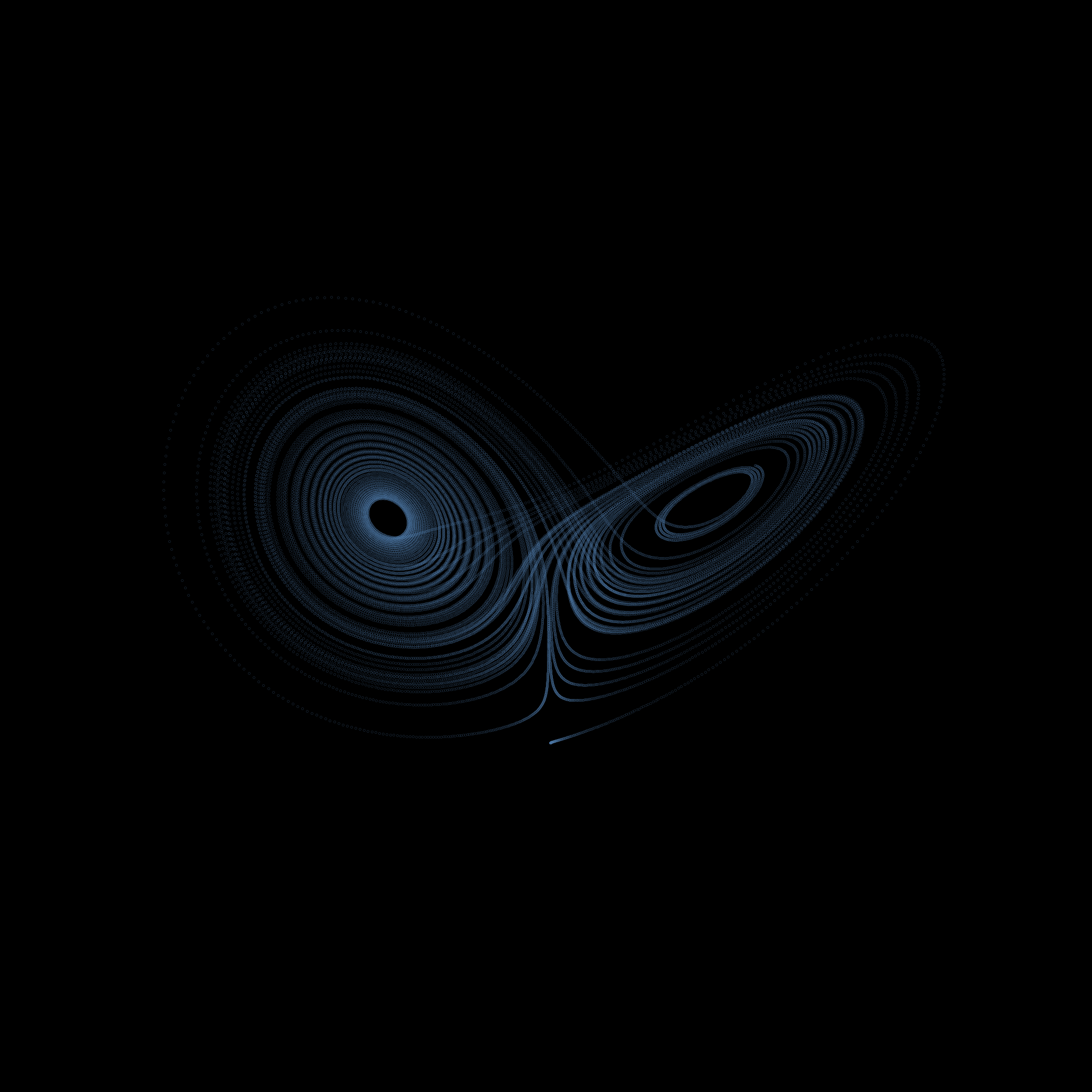
Because of its striking visual when plotted it’ll serve as a good example to show how animplotlib can be used for creating a more complex animation. A standout property of chaotic systems is that they’re very sensitive to changes in their input parameters. We can visualise this by plotting the Lorenz attractor with various initial conditions on the same axes.

First we import the necessary libraries and then create a list of initial conditions we’ll be solving over. We do this by adding a tiny $\epsilon$ to an initial condition. We can also create two functions: one for defining the Lorenz system and one for solving it.

import matplotlib.pyplot as plt
from scipy.integrate import odeint
import numpy as np
import animplotlib as anim

t = np.linspace(0.01, 50, 5000)
# Distinct colours for each trajectory
colours = [
    "#4E79A7",
    "#F28E2B",
    "#46ACB8",
    "#E15759",
    "#4E79A7",
    "#F28E2B",
    "#4E79A7",
    "#F28E2B",
    "#46ACB8",
    "#E15759",
    "#4E79A7",
    "#F28E2B",
    "#4E79A7",
    "#4E79A7",
    "#F28E2B",
    "#F28E2B",
]
# List of initial conditions
epsilon = 1e-5
x0 = [(10.0, 10.0, 10.0 + n * epsilon) for n in range(len(colours))]


# Defining the Lorenz system
def lorenz(x_var, t, sigma, rho, beta):
    x, y, z = x_var
    dx_dt = sigma * (y - x)
    dy_dt = x * (rho - z) - y
    dz_dt = x * y - beta * z
    return [dx_dt, dy_dt, dz_dt]

# Solving the system
def solve_lorenz(x0, t, sigma, rho, beta):
    return odeint(lorenz, x0, t, args=(sigma, rho, beta))

Next we create a figure and axes, and empty lists for the lines, points and data points to be passed to animplotlib:

fig = plt.figure(figsize=(8, 8))
ax = fig.add_subplot(111, projection='3d')
ax.set_axis_off()

# Lists to hold lines, points, and data for each trajectory
lines = []
points = []
xs, ys, zs = [], [], []

Here, we iterate over the initial conditions we defined earlier and call the solve_lorenz function to solve for each set of initial conditions. We also apply a different colour to each solution to more easily differentiate between them. Then, we create a line and point for each solution and append it to the corresponding list to be passed to AnimPlot3D.

# Solve for each set of initial conditions and create a line and point for each
for init_cond, colour in zip(x0, colours):
    x_solve = solve_lorenz(init_cond, t, sigma=10, rho=28, beta=8/3)
    x, y, z = x_solve.T
    xs.append(x)
    ys.append(y)
    zs.append(z)
    line, = ax.plot([], [], [], lw=2, color=colour)
    point, = ax.plot([], [], [], 'o', color=colour, markersize=10)
    lines.append(line)
    points.append(point)

ax.set_xlim(np.min(xs), np.max(xs))
ax.set_ylim(np.min(ys), np.max(ys))
ax.set_zlim(np.min(zs), np.max(zs))

# Call the AnimPlot3D class
anim.AnimPlot3D(fig, [ax] * len(lines), lines, points, xs, ys, zs, plot_speed=1,
           rotation_speed=0.25, l_num=100, p_num=1)

Note that when passing the axes to AnimPlot3D we multiply the list by len(lines). This is because AnimPlot3D expects a list of axes, one for each line/trajectory we want to animate. Passing just [ax] (a single axis) would result in only the first line/trajectory being animated. By passing [ax] * len(lines), we create a list with the same axis repeated for each line, allowing all lines to be animated.

Notice how initially it looks as though there is only one solution being plotted with all the solutions overlapping. As the time steps progress the solutions begin to spread. Remember the initial conditions for each solution only differ by $0.000001$, and even then each solution begins to take its own unique trajectory.

Back to examples