Mass transport by diffusion Deriving an expression for the concentration profile for semi-transient
5 Aug 2024 · 4 min read
Given some medium, e.g. water,
containing some material, say salt, the material will DIFFUSE from the
concentrated area to the dilute area. Diffusion can be generalised by Fick’s law:
J = − D d C d x J = -D \frac{\text{d} C}{\text{d} x} J = − D d x d C
where J J J D D D δ t \delta t δ t
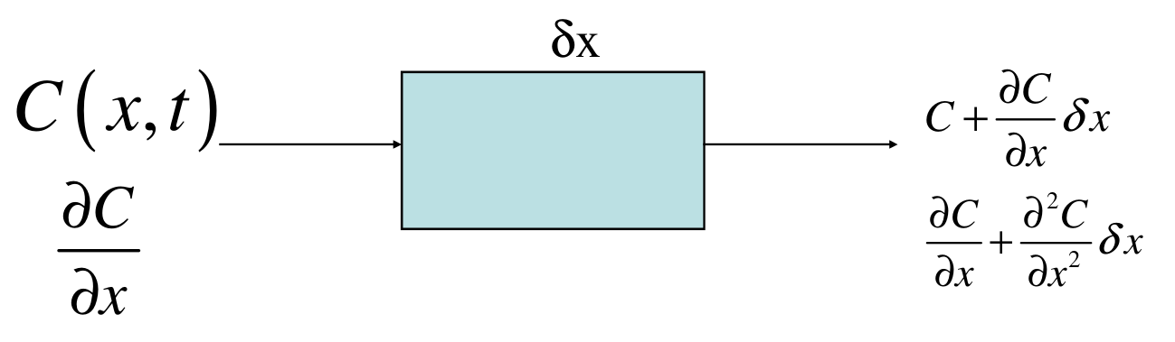
MOLES IN − MOLES OUT = Accumulated MOLES \text{MOLES IN} - \text{MOLES OUT} = \text{Accumulated MOLES} MOLES IN − MOLES OUT = Accumulated MOLES − D ∂ C ∂ x A δ t − [ − D ( ∂ C ∂ x + ∂ 2 C ∂ x 2 δ x ) ] A δ t = V Δ C . -D\frac{\partial C}{\partial x} A \delta t - \left[ -D \left( \frac{\partial
C}{\partial x} + \frac{\partial^2 C}{\partial x^2}\delta x \right) \right]
A\delta t = V\Delta C. − D ∂ x ∂ C A δ t − [ − D ( ∂ x ∂ C + ∂ x 2 ∂ 2 C δ x ) ] A δ t = V Δ C . Replacing V = A δ x V = A\delta x V = A δ x
− D ∂ C ∂ x A δ t − [ − D ( ∂ C ∂ x + ∂ 2 C ∂ x 2 δ x ) ] A δ t = A δ x Δ C . -D\frac{\partial C}{\partial x} A \delta t - \left[ -D \left( \frac{\partial
C}{\partial x} + \frac{\partial^2 C}{\partial x^2}\delta x \right) \right]
A\delta t = A\delta x \Delta C. − D ∂ x ∂ C A δ t − [ − D ( ∂ x ∂ C + ∂ x 2 ∂ 2 C δ x ) ] A δ t = A δ x Δ C . − D ∂ C ∂ x A δ t + D ( ∂ C ∂ x + ∂ 2 C ∂ x 2 δ x ) A δ t = A δ x Δ C . -D\frac{\partial C}{\partial x} A \delta t + D\left( \frac{\partial
C}{\partial x} + \frac{\partial^2 C}{\partial x^2}\delta x \right)
A\delta t = A\delta x \Delta C. − D ∂ x ∂ C A δ t + D ( ∂ x ∂ C + ∂ x 2 ∂ 2 C δ x ) A δ t = A δ x Δ C . − D ∂ C ∂ x + D ∂ C ∂ x + D ∂ 2 C ∂ x 2 δ x = δ x Δ C δ t . -D\frac{\partial C}{\partial x} + D\frac{\partial
C}{\partial x} + D\frac{\partial^2 C}{\partial x^2}\delta x
= \delta x \frac{\Delta C}{\delta t}. − D ∂ x ∂ C + D ∂ x ∂ C + D ∂ x 2 ∂ 2 C δ x = δ x δ t Δ C . D ∂ 2 C ∂ x 2 = Δ C δ t . D\frac{\partial^2 C}{\partial x^2}= \frac{\Delta C}{\delta
t}. D ∂ x 2 ∂ 2 C = δ t Δ C . Taking the limit as the right hand side goes the zero we see that the above
equation approaches
∂ C ∂ t = D ∂ 2 C ∂ x 2 \frac{\partial C}{\partial t} = D \frac{\partial^2 C}{\partial x^2} ∂ t ∂ C = D ∂ x 2 ∂ 2 C This is the 1D diffusion equation over a small control volume V V V
Let us consider the case of transient diffusion through a semi-infinite
geometry. The boundary conditions in this case are
at t < 0 t < 0 t < 0 C A = C A , i , C_{A} = C_{A,i}, C A = C A , i ,
at t > 0 t > 0 t > 0 C A → C A , i C_{A} \to C_{A,i} C A → C A , i x = 0 x = 0 x = 0
at t > 0 t > 0 t > 0 C A = C A , s C_{A} = C_{A,s} C A = C A , s
Let us define a similarity variable, η \eta η x x x t t t
η = x 4 D t \eta = \frac{x}{\sqrt{4Dt}} η = 4 D t x We can now re-write the diffusion equation in terms of the similarity variable.
∂ C ∂ x = ∂ C ∂ η ∂ η ∂ x \frac{\partial C}{\partial x} = \frac{\partial C}{\partial \eta}\frac{\partial \eta}{\partial x} ∂ x ∂ C = ∂ η ∂ C ∂ x ∂ η ∂ η ∂ x = 1 4 D t \frac{\partial \eta}{\partial x} = \frac{1}{\sqrt{4Dt}} ∂ x ∂ η = 4 D t 1 And so, in terms of η \eta η
∂ C ∂ x = 1 4 D t ∂ C ∂ η \frac{\partial C}{\partial x} = \frac{1}{\sqrt{4Dt}}\frac{\partial C}{\partial \eta} ∂ x ∂ C = 4 D t 1 ∂ η ∂ C The second derivative term can be broken up as
∂ 2 C ∂ x 2 = ∂ ∂ x ( ∂ C ∂ x ) = ∂ ∂ x ( d C d η ⋅ d η d x ) = ∂ 2 C ∂ η 2 d η d x ⋅ d η d x = 1 4 D t ∂ 2 C ∂ η 2 \begin{equation*}
\begin{aligned}
\frac{\partial^2 C}{\partial x^2} &= \frac{\partial}{\partial x}\left(\frac{\partial C}{\partial x}\right) \\
&= \frac{\partial}{\partial x}\left(\frac{\text{d} C}{\text{d} \eta}\cdot\frac{\text{d} \eta}{\text{d} x}\right) \\
&= \frac{\partial^2 C}{\partial \eta^2} \frac{\text{d}\eta}{\text{d} x}\cdot\frac{\text{d}\eta}{\text{d} x} \\
&= \frac{1}{4Dt} \frac{\partial^2 C}{\partial \eta^2}
\end{aligned}
\end{equation*} ∂ x 2 ∂ 2 C = ∂ x ∂ ( ∂ x ∂ C ) = ∂ x ∂ ( d η d C ⋅ d x d η ) = ∂ η 2 ∂ 2 C d x d η ⋅ d x d η = 4 D t 1 ∂ η 2 ∂ 2 C Taking the derivative of η \eta η
∂ η ∂ t = x 4 D ⋅ − t − 3 2 2 = − x 2 t 4 D t \begin{equation*}
\begin{aligned}
\frac{\partial \eta}{\partial t} &= \frac{x}{4D}\cdot\frac{-t^{-\frac{3}{2}}}{2} \\
&= -\frac{x}{2t\sqrt{4Dt}}
\end{aligned}
\end{equation*} ∂ t ∂ η = 4 D x ⋅ 2 − t − 2 3 = − 2 t 4 D t x and so,
∂ C ∂ t = d C d η d η d t = d C d η ( − x 2 t 4 D t ) \begin{equation*}
\begin{aligned}
\frac{\partial C}{\partial t} &= \frac{\text{d} C}{\text{d} \eta}
\frac{\text{d} \eta}{\text{d} t} \\
&= \frac{\text{d} C}{\text{d} \eta}\left(-\frac{x}{2t\sqrt{4Dt}}\right)
\end{aligned}
\end{equation*} ∂ t ∂ C = d η d C d t d η = d η d C ( − 2 t 4 D t x ) The diffusion equation thus becomes
1 4 D t ∂ 2 C ∂ η 2 = 1 D d C d η ( − x 2 t 4 D t ) d 2 C d η 2 = − 2 x 4 D t d C d η \begin{equation*}
\begin{aligned}
\frac{1}{4Dt}\frac{\partial^2 C}{\partial \eta^2} &= \frac{1}{D}\frac{\text{d}C}{\text{d}\eta}\left(-\frac{x}{2t\sqrt{4Dt}}\right) \\
\frac{\text{d}^2 C}{\text{d} \eta^2} &=
-\frac{2x}{\sqrt{4Dt}}\frac{\text{d}C}{\text{d}\eta}
\end{aligned}
\end{equation*} 4 D t 1 ∂ η 2 ∂ 2 C d η 2 d 2 C = D 1 d η d C ( − 2 t 4 D t x ) = − 4 D t 2 x d η d C Since x = η 4 D t x = \eta\sqrt{4Dt} x = η 4 D t
d 2 C d η = − 2 η d C d η \begin{equation*}
\begin{aligned}
\frac{\text{d}^2 C}{\text{d} \eta} = -2\eta \frac{\text{d} C}{\text{d} \eta}
\end{aligned}
\end{equation*} d η d 2 C = − 2 η d η d C Rewriting the boundary conditions in terms of η \eta η
C A = C A , i C_{A} = C_{A, i} C A = C A , i t = 0 ∴ η → ∞ t = 0 \ \therefore \ \eta \to \infty t = 0 ∴ η → ∞ C A = C A , s C_{A} = C_{A, s} C A = C A , s t > 0 ∴ η = 0 t > 0 \ \therefore \ \eta = 0 t > 0 ∴ η = 0 C A = C A , i C_{A} = C_{A, i} C A = C A , i t > 0 t > 0 t > 0 x → ∞ ∴ η = 0 x \to \infty \ \therefore \ \eta = 0 x → ∞ ∴ η = 0
The similarity variable combines the variables x x x t t t η \eta η C C C U = d C d η U = \frac{\text{d}C}{\text{d}\eta} U = d η d C
d U d η = − 2 η U \begin{equation*}
\begin{aligned}
\frac{\text{d} U}{\text{d} \eta} = - 2\eta U
\end{aligned}
\end{equation*} d η d U = − 2 η U and now integrating both sides,
ln U = − η 2 + C 0 U = C 1 e − η 2 \begin{equation*}
\begin{aligned}
\ln U &= -\eta^2 + C_0 \\
U &= C_1e^{-\eta^2}
\end{aligned}
\end{equation*} ln U U = − η 2 + C 0 = C 1 e − η 2 Substituting back in for U U U C C C
d C d η = C 1 e − η 2 C = C 1 ∫ e − η 2 d η + C 2 \begin{equation*}
\begin{aligned}
\frac{\text{d} C}{\text{d} \eta} &= C_1e^{-\eta^2} \\
C &= C_1\int e^{-\eta^2} \text{d}\eta + C_2
\end{aligned}
\end{equation*} d η d C C = C 1 e − η 2 = C 1 ∫ e − η 2 d η + C 2 Applying the boundary conditions:
C ( η = 0 ) = C s ⇒ C 2 = C s C(\eta = 0) = C_s \Rightarrow C_2 = C_s C ( η = 0 ) = C s ⇒ C 2 = C s C ( η → ∞ ) = C i ⇒ C i = C 1 ∫ 0 ∞ e − η 2 d η + C s C(\eta \to \infty) = C_i \Rightarrow C_i = C_1\int_0^\infty e^{-\eta^2}
\text{d} \eta + C_s C ( η → ∞ ) = C i ⇒ C i = C 1 ∫ 0 ∞ e − η 2 d η + C s
The above integral is half the Gaussian integral which can be evaluated to
π 2 \frac{\sqrt{\pi}}{2} 2 π C 1 C_1 C 1
C i = π 2 C 1 + C s C 1 = 2 π ( C i − C s ) \begin{equation*}
\begin{aligned}
C_i = \frac{\sqrt{\pi}}{2}C_1 + C_s \\
C_1 = \frac{2}{\sqrt{\pi}}(C_i - C_s)
\end{aligned}
\end{equation*} C i = 2 π C 1 + C s C 1 = π 2 ( C i − C s ) And so, we get the expression for C C C
C = 2 π ( C i − C s ) ∫ 0 η e − η 2 d η + C s C − C s C i − C s = 2 π ∫ 0 η e − η 2 d η \begin{equation*}
\begin{aligned}
C = \frac{2}{\sqrt{\pi}}(C_i - C_s)&\int_0^\eta e^{-\eta^2} \text{d} \eta + C_s
\\
\frac{C - C_s}{C_i - C_s} = \frac{2}{\sqrt{\pi}}&\int_0^\eta
e^{-\eta^2}\text{d}\eta
\end{aligned}
\end{equation*} C = π 2 ( C i − C s ) C i − C s C − C s = π 2 ∫ 0 η e − η 2 d η + C s ∫ 0 η e − η 2 d η The integral ∫ 0 η e − η 2 d η \int_0^\eta e^{-\eta^2} \text{d} \eta ∫ 0 η e − η 2 d η η → ∞ \eta \to \infty η → ∞ error function can be defined as
erf ( η ) ≡ 2 π ∫ 0 η e − η 2 d η \begin{equation*}
\begin{aligned}
\text{erf}(\eta) \equiv \frac{2}{\sqrt{\pi}} \int_0^\eta e^{-\eta^2} \text{d}
\eta
\end{aligned}
\end{equation*} erf ( η ) ≡ π 2 ∫ 0 η e − η 2 d η with erf ( 1 ) = 1 \text{erf}(1) = 1 erf ( 1 ) = 1 erf ( 0 ) = 0 \text{erf}(0) = 0 erf ( 0 ) = 0
C − C s C i − C s = erf ( η ) \begin{equation*}
\begin{aligned}
\boxed{
\frac{C - C_s}{C_i - C_s} = \text{erf}(\eta)
}
\end{aligned}
\end{equation*} C i − C s C − C s = erf ( η )