Visualising some interesting strange attractors

---

Lorenz attractor

The most well known attractor is the Lorenz attractor. This was discovered by Edward Lorenz in the 1960s while he was trying to create a mathematical model to describe the behaviour of convection cells in the Earth’s atmosphere. He developed a system of three non-linear differential equations that represented the flow of air within a simplified atmospheric model, with the aim of capturing the complex dynamics of convection.

\[\left\{ \begin{array}{ll} \frac{dx}{dt}&=&\sigma (-x + y)\\ \frac{dy}{dt}&=& -x z + \rho x - y \\ \frac{dz}{dt}&=& x y - \beta z \end{array} \right.\]

Using early computers he was able to carry out numerical simulations of the equations. In these simulations he noticed that with smallest of changes to the initial conditions, the trajectories of the solutions would diverge dramatically over time. He famously described this as the “butterfly effect”, underscoring the extreme sensitivity of chaotic systems to initial conditions. Lorenz’s work fundamentally changed the understanding of deterministic chaos and influenced the development of chaos theory and the study of non-linear dynamical systems in the various scientific disciplines.

The classic butterfly shaped solution curve is achieved when $\rho = 28, \ \sigma = 10$ and $\beta = 8/3$, and initial conditions such as $[0, 1, 15]$.

De Jong attractor

The De Jong attractor can be characterised by the following equations

\[x_{n+1} = \sin(a y_n) - \cos(b x_n) \\ y_{n+1} = \sin(c x_n) - \cos(d y_n),\]

Here $a,\ b,\ c$ and $d$ are constants. Generating $(x,y)$ coordinates over many iterations results in some striking visualisations of the attractor

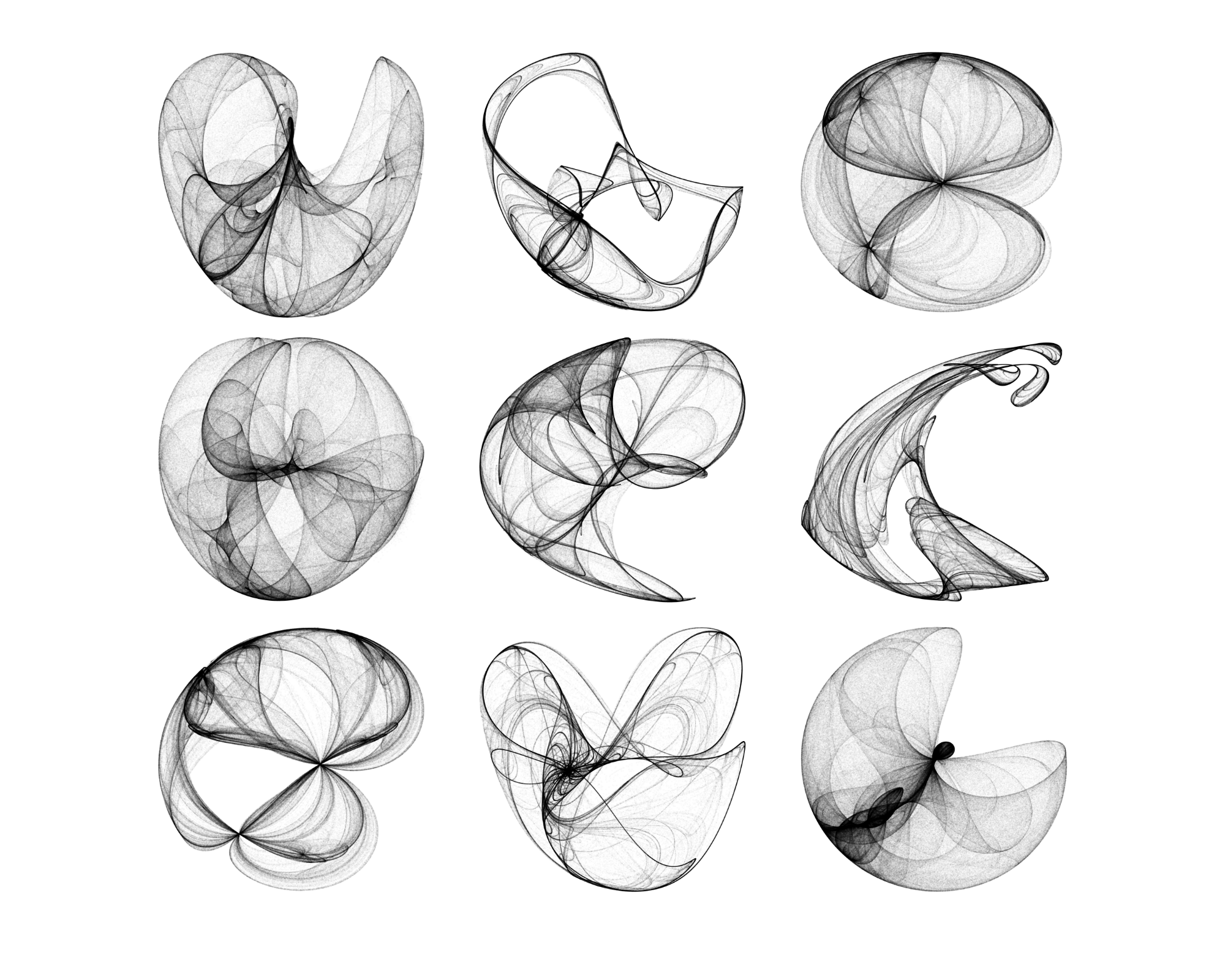
The above plots have the same initial conditions for $x$ and $y$ but show how changing the values of the parameters $a,\ b,\ c$ and $d$ affects the system.

Clifford attractor

A variation of the De Jong attractor is the Clifford attractor:

\[x_{n+1} = \sin(a y_n) + c \cos(b x_n) \\ y_{n+1} = \sin(c x_n) + d \cos(d y_n),\]

Similar to the De Jong attractor, varying the constants $a,\ b,\ c$ and $d$ with set initial conditions, and plotting $x$ and $y$ over a large number of iterations leads to some cool looking plots.

Other attractors

The discovery of the Lorenz attractor prompted the emergence of a large number of chaotic systems in various disciplines. These new chaotic systems take on different topological structures i.e. one-scroll, multi-scroll, butterfly, multi-wing. Some of these are Visualised below.

Aizawa

The Aizawa attractor, names after Akira Aizawa is described by the following set of differential equations:

\[\left\{ \begin{array}{ll} \frac{dx}{dt}&=&(z - b) x - d y\\ \frac{dy}{dt}&=& d x + (z - b) y\\ \frac{dz}{dt}&=&c + a z - \frac{z^3}{3} -\\& &\;(x^2+y^2)(1+e z)+f z x^3 \end{array} \right.\]

The above visualisations correspond to parameter values of $a = 1,\ b = 0.7,
c = 0.6,\ d = 3.5,\ e = 0.25,\ f = 0.1$.

Three-scroll

\[\left\{ \begin{array}{ll} \frac{dx}{dt}&=& y + a x y +x z \\ \frac{dy}{dt}&=& 1 - b x^2 +yz \\ \frac{dz}{dt}&=& x-x^2-y^2 \end{array} \right.\]

The above visualisations correspond to parameter values of $a = 1,\ b = 0.7,
c = 0.6,\ d = 3.5,\ e = 0.25,\ f = 0.1$.

Thomas attractor

\[\left\{ \begin{array}{ll} \frac{dx}{dt}&=&\sin y -bx\\ \frac{dy}{dt}&=&\sin z -by\\ \frac{dz}{dt}&=&\sin x-bz \end{array} \right.\]

The above visualisations correspond to parameter values of $a = 1,\ b = 0.7,
c = 0.6,\ d = 3.5,\ e = 0.25,\ f = 0.1$.

Multi-wing attractors

Dadras

\[\left\{ \begin{array}{ll} \frac{dx}{dt}&=& y - a x +b y z\\ \frac{dy}{dt}&=& c y - x z +z\\ \frac{dz}{dt}&=& d x y - e z \end{array} \right.\]

The above visualisations correspond to parameter values of $a = 1,\ b = 0.7,
c = 0.6,\ d = 3.5,\ e = 0.25,\ f = 0.1$.