Torus knots are a class of knots that lie on and wrap around the surface of a torus.

Because it produces a cool looking plot we’ll use the torus knot as a slightly more complex example of using animplotlib. This will be similar to creating the lorenz attractor animation where we made multiple plots on a single axes. Here, however, we’ll create three animations, each on its own axis within the same figure.

Torus knots are defined parametrically by the following set of equations:

$x(t) = (R + \cos(pt))(\cos(qt))$

$y(t) = (R + \cos(pt))(\sin(qt))$

$z(t) = -\sin(pt)$

where $R$ is the radius of the torus (think of this as its “thickness”) and $p$ and $q$ are integers which must be coprime. This is important as it allows the torus to form a single, continuous loop. A common configuration to view the torus knot is with $R = 2$. For the parameters $p$ and $q$ we’ll use three different pairs: $(3, 2)$, $(7, 3)$ and $(15, 4)$. Once animated, we’ll be able to get a better idea as to how these parameters determine the shape of their respective knots.

We can start with importing the necessary libraries, defining the knot and the values for $p$ and $q$. We’ll allow $t$ to run over a period of $0$ to $2\pi$ (i.e. one whole revolution).

import numpy as np
import matplotlib.pyplot as plt
import animplotlib as anim

n = 1000
t = np.linspace(0, 2 * np.pi, n)

parameters = [(3, 2), (7, 3), (15, 4)]
colours = ['#46ACB8', '#F28E2B', '#E15759']


def torus(p, q):
    x = (2 + np.cos(p * t)) * (np.cos(q * t))
    y = (2 + np.cos(p * t)) * (np.sin(q * t))
    z = -np.sin(p * t)
    return x, y, z

We can create a figure as well as some empty lists to store the axes, lines, points and the data we’ll be plotting.

fig = plt.figure(figsize=(10, 5))
axes = []
lines = []
points = []
xs, ys, zs = [], [], []

Next, we call the $\texttt{torus}$ function for each set of parameters we defined earlier. We can then create a line, point and static plot and append each of these to the corresponding lists created above.

for parameter, colour in zip(parameters, colours):
    p, q = parameter
    x, y, z = torus(p, q)
    xs.append(x)
    ys.append(y)
    zs.append(z)

    ax = fig.add_subplot(1, 3, len(axes) + 1, projection='3d')
    axes.append(ax)
    ax.plot(x, y, z, c=colour)
    line, = ax.plot([], [], [], lw=0)
    point, = ax.plot([], [], [], 'o', c=colour, markersize=10)
    lines.append(line)
    points.append(point)

    ax.set_xlim(np.min(x), np.max(x))
    ax.set_ylim(np.min(y), np.max(y))
    ax.set_zlim(np.min(z), np.max(z))
    ax.set_axis_off()

# Calling the AnimPlot3D class
anim.AnimPlot3D(fig, axes, lines, points, xs, ys, zs, plot_speed=2,
                rotation_speed=0.36)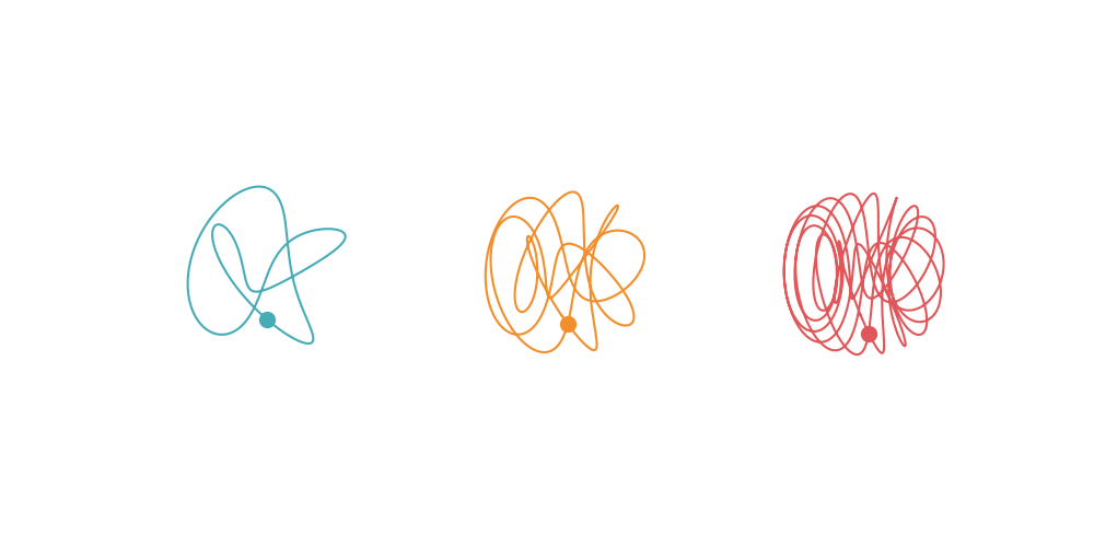

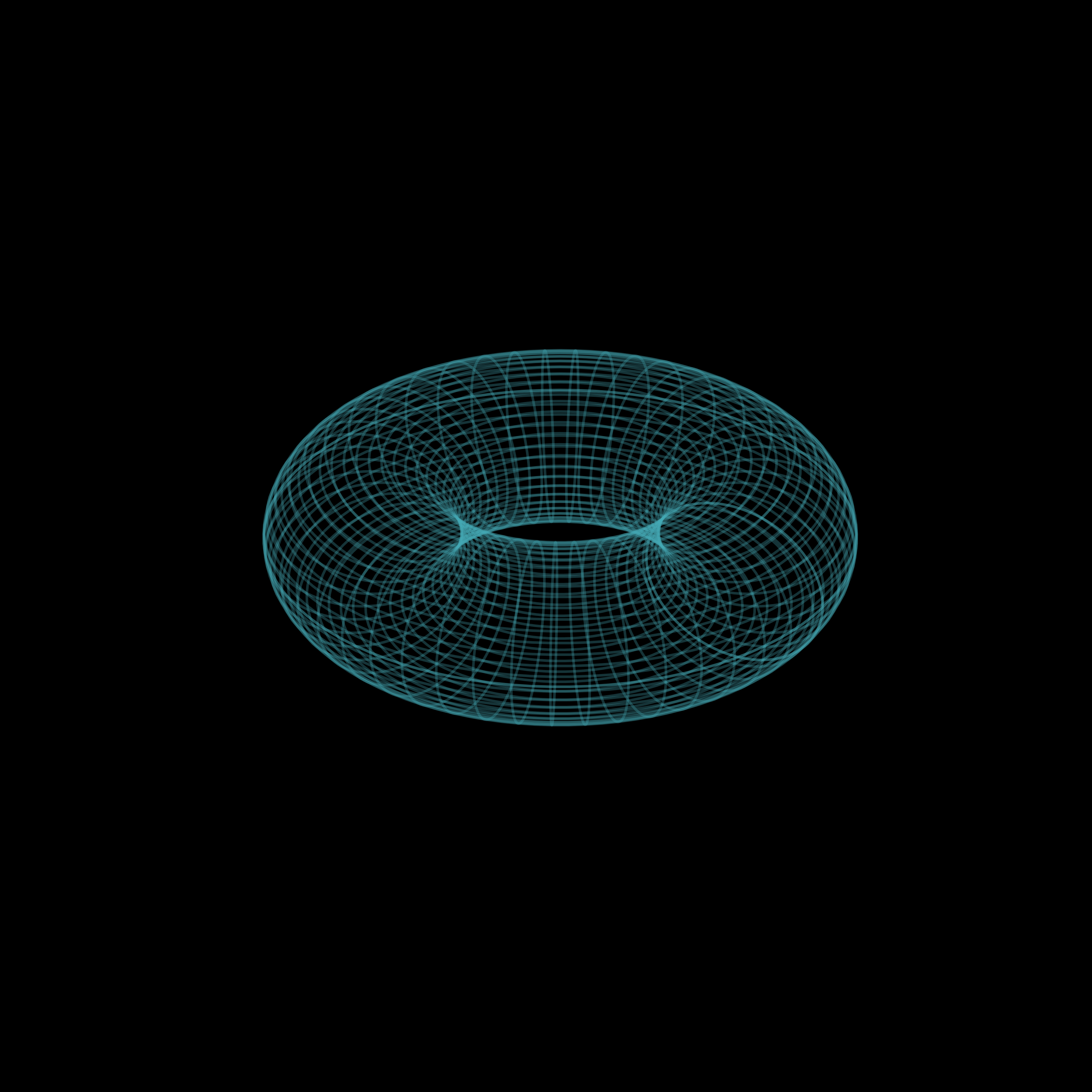
We can see from the animation how the density and complexity of the knot increases as we change the values of $p$ and $q$. Let’s overlay the knot with $p = 7$ and $q = 3$ to better see how these parameters relate to a torus:

Staring at this for a while you may begin to see that the knot actually loops around the torus 7 times (i.e. $p$ times) and around its central axis 3 times (i.e. $q$ times). Creating these animations makes it a lot easier to understand what these parameters actually mean in the context of the equations and how the knot is affected as we change them.

Back to examples